Functional connectivity analyses¶

We have examined evoked BOLD responses and spatial patterns of activity, but sometimes information can be represented more globally at a network level. One measure of interactions between brain areas that are physically distant is functional connectivity. Functional connectivity is usually measured by a Pearson correlation between the BOLD time courses extracted from two distinct areas in the brain. In this section, we will demonstrate basic steps for functional connectivity analyses by using the ‘story’ task data from the sample dataset.

This section is developed based on the Intro to Functional Connectivity workbook designed by Michael Arcaro as part of NEU502.

Confound regression¶

Confound regression is crucial for functional connectivity analyses because connectivity measures are affected by artifacts that systematically shape BOLD timeseries, such as head motion, scanner-induced artifacts, respiratory artifacts, etc. Unfortunately, there is no gold standard for confound regression (i.e. which variables to regress out, whether to use scrubbing), but there is much information about pros and cons of different pipelines [e.g., Parkes et al. 2018, Ciric et al. 2017].

Here, we demonstrate one procedure to perform confound regression (also see this page). We assume you have followed the instructions for fMRIPrep and preprocessed the data already. Let’s take the preprocessed data (i.e., fMRIPrep-ed data). For each run, extract regressor columns from the confounds_regressors.tsv file. You can regress out CSF, WM, global signal, and motion (e.g., 6-, 12-, 24-parameter), aCompCor components, and/or AROMA outputs.

Preprocessed BOLD data (in MNI space) and confound regressors for each run:

func_file=BIDS_DIR/derivatives/fmriprep/sub-001/ses-01/func/sub-001_ses-01_task-story_run-1_space-MNI152NLin2009cAsym_desc-preproc_bold.nii.gz
confound_file=BIDS_DIR/derivatives/fmriprep/sub-001/ses-01/func/sub-001_ses-01_task-story_run-1_desc-confounds_regressors.tsv

Extract confound regressor columns and save to a 1D file, using AFNI’s 1dcat:

module load afni
1dcat $confound_file'[HEADER1, HEADER2,...]' > confounds_ortvec_run-1.1D

The following code performs confound regression, spatial/temporal smoothing, and censoring in a single step, using AFNI’s 3dTproject. Here, we demonstrate how to include polynomial orthogonalization (-polort 2), confound regressors (-ort FILENAME), spatial smoothing with a 4mm kernel (-blur 4), bandpass filtering (-bandpass 0.01 0.1), and censoring (-censor and -cenmode). Feel free to include a subset of these options.

3dTproject \
-polort 2 \
-input $func_file \
-ort confounds_ortvec_run-1.1D \
-blur 4 \
-bandpass 0.01 0.1 \
-censor CENSOR_FILE -cenmode ZERO \
-prefix OUTPUT_FILENAME

Here’s a sample script to repeat the steps above for all four runs and concatenate them. This script filters out CSF, WM, global signal, and 24-parameter motion and does not perform any temporal/spatial smoothing or censoring.

#! /bin/bash

module load afni

PROJECT_DIR=/jukebox/YOURLAB/USERNAME/sample_project
BIDS_DIR=$PROJECT_DIR/data/bids

# set paths to your directories
func_dir=$BIDS_DIR/derivatives/fmriprep/sub-001/ses-01/func
out_dir=[your output directory]

# confound regression
for runidx in 1 2 3 4
do
        # for each run, extract columns of interest from the confounds file
        confoundfile=$func_dir/sub-001_ses-01_task-story_run-0${runidx}_desc-confounds_regressors.tsv
        1dcat $confoundfile'[csf,white_matter,global_signal,trans_x,trans_x_derivative1,trans_x_derivative1_power2,trans_x_power2,trans_y,trans_y_derivative1,trans_y_derivative1_power2,trans_y_power2,trans_z,trans_z_derivative1,trans_z_derivative1_power2,trans_z_power2,rot_x,rot_x_derivative1,rot_x_derivative1_power2,rot_x_power2,rot_y,rot_y_derivative1,rot_y_power2,rot_y_derivative1_power2,rot_z,rot_z_derivative1,rot_z_derivative1_power2,rot_z_power2]' > $out_dir/confounds_ortvec_run-0${runidx}.1D

        #  regress out and save the 'denoised' file into the output directory
        3dTproject -polort 2 -input $func_dir/sub-001_ses-01_task-story_run-0${runidx}_space-MNI152NLin2009cAsym_desc-preproc_bold.nii.gz        \
                   -ort $out_dir/confounds_ortvec_run-0${runidx}.1D \
                   -prefix $out_dir/sub-001_ses-01_task-story_run-0${runidx}_space-MNI152NLin2009cAsym_desc-denoised.nii.gz
done

# concatenate all four runs into a single file
3dTcat -prefix $out_dir/sub-001-denoised.nii.gz \
           $out_dir/sub-001_ses-01_task-story_run-01_space-MNI152NLin2009cAsym_desc-denoised.nii.gz \
           $out_dir/sub-001_ses-01_task-story_run-02_space-MNI152NLin2009cAsym_desc-denoised.nii.gz \
           $out_dir/sub-001_ses-01_task-story_run-03_space-MNI152NLin2009cAsym_desc-denoised.nii.gz \
           $out_dir/sub-001_ses-01_task-story_run-04_space-MNI152NLin2009cAsym_desc-denoised.nii.gz

# copy T1w image for visualization
cp [sample_project directory]/data/bids/derivatives/fmriprep/sub-001/anat/sub-001_space-MNI152NLin2009cAsym_desc-preproc_T1w.nii.gz $out_dir

Seed-based exploration¶

AFNI provides a way of exploring functional connectivity in your dataset through a simple seed-based correlation analysis via the InstaCorr program.

Go to your output directory, and launch AFNI. .. code-block:: bash

$ cd [output directory] $ afni &

In the AFNI window, click on ‘UnderLay’ and select the anatomical image copied from the BIDS directory (“sub-001_space-MNI152NLin2009cAsym_desc-preproc_T1w.nii.gz”).

Click ‘Define Overlay’ to expand the window.
Click on the ‘Setup ICorr’ in top right corner to reveal this new window:

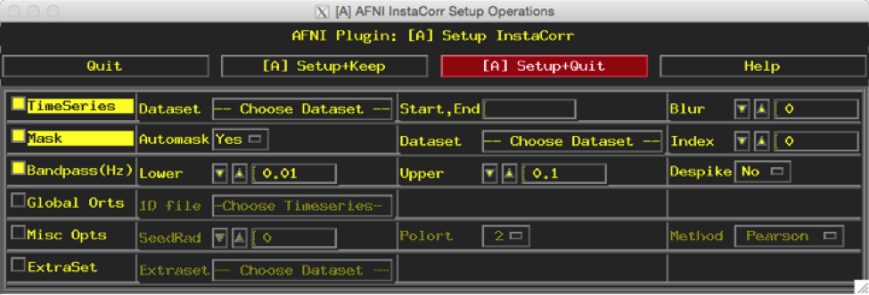
Select ‘Choose Dataset’ & Select ‘sub-001-denoised.nii.gz’
Increase ‘Blur’ to 4
In the ‘Mask’ row, change ‘Automask’ to No
Use the default Bandpass setup (Lower 0.01; Upper 0.1) since bandpass filtering was not done on the data.
Click ‘[A] Setup+Keep’ (DO NOT CLICK AROUND WHILE RUNNING!)
Wait for correlations to finish. You should see this line in the terminal: ++ InstaCorr setup: 245245 voxels ready for work
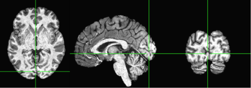
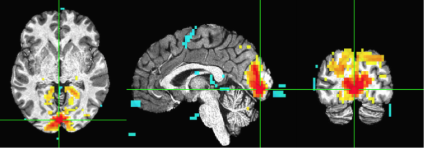
In the anatomical image, move the cursor to the point you want to test. For example, I moved the cursor to a point in the primary visual cortex.

Near the cursor, right click (and hold) in any window to reveal a hidden drop down menu.
Select ‘InstaCorr Set’
Change threshold in main window to .3

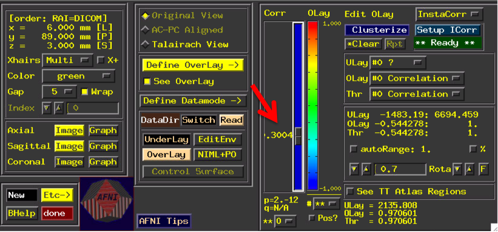
You should see a correlation pattern that looks like this:

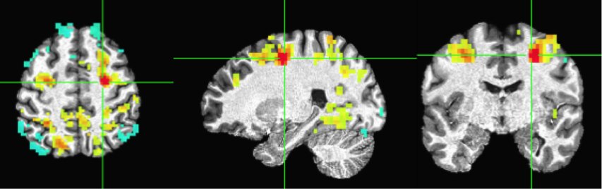
Move the cursor to another point. Here I selected a point from the frontoparietal attention network (or “Dorsal Attention Network”). And redo ‘InstalCorr Set’. Then you will see the network revealted (as positively correlated) in this subject, as well as some anti-correlated regions. Feel free to play around with the threshold (higher or lower).

There are a few other options that you can try in the Setup InstaCorr window, such as Blur and SeedRad (you need to check ‘Misc Opts’). Change the options and rerun the correlations by clicking ‘[A] Setup+Keep’.

Pairwise connectivity between ROIs¶

We are going to create two spherical ROIs by using the procedures described in Andy’s Brain Blog.

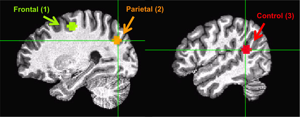
For practice, we will choose one ROI in the frontal lobe and another ROI in the parietal lobe, which are highly correlated (both areas are part of the so-called Dorsal Attention Network). As a control, we will choose one additional area in the parietal-temporal lobe that is not part of the same network. All these ROIs are in the right hemisphere (this is why there is a little ‘r’ in the file name).

In your output directory, make a text file for each of the following coordinates:

rFrontal.txt .. code-block:: bash

28 -9 53

rParietal.txt .. code-block:: bash

28 -71 32

rControl.txt .. code-block:: bash

51 -47 17

Create spherical ROIs around those coordinates using AFNI’s 3dUndump: .. code-block:: bash

3dUndump -prefix rFrontal -master sub-001-denoised.nii.gz -srad 6 -xyz rFrontal.txt 3dUndump -prefix rParietal -master sub-001-denoised.nii.gz -srad 6 -xyz rParietal.txt 3dUndump -prefix rControl -master sub-001-denoised.nii.gz -srad 6 -xyz rControl.txt

Basic input and options: * -prefix specify output filename * -master specify a reference file. ROIs will use the same grid information. Because we will extract BOLD timeseries, the code above uses the BOLD file (output of 3dTproject). * -srad radius, size of the spherical ROI (in mm) * -xyz coordinate of the ROI

Visually inspect whether your ROIs are created in the right location:

Extract time courses (across the four runs) from the three ROIs and save each into a 1D file. .. code-block:: bash

3dmaskave -mask rFrontal+tlrc sub-001-denoised.nii.gz > rFrontal-denoised.1D 3dmaskave -mask rParietal+tlrc sub-001-denoised.nii.gz > rParietal-denoised.1D 3dmaskave -mask rControl+tlrc sub-001-denoised.nii.gz > rControl-denoised.1D

Now you have BOLD timeseries extracted from each ROI. You can load these files in MATLAB, Python, R, etc. and calculate Pearson correlations between each of the possible pairs.

Computing correlation matrices from a set of ROIs¶

Combine ROIs into a map and assign each of the ROIs a different value (1 = rFrontal, 2 = rParietal, 3 = rControl).

3dcalc \
-a rFrontal+tlrc \
-b rParietal+tlrc \
-c rControl+tlrc \
-expr 'a+b*2+c*3' \
-prefix ROImap

Calculate a correlation matrix from the ROI map

3dNetCorr \
-inset sub-001-denoised.nii.gz \
-in_rois ROImap+tlrc \
-fish_z \
-ts_wb_corr \
-prefix ROImap_matrix

Basic input and options: * -inset BOLD data file * -in_rois A map of ROIs. You can also use a whole-brain parcellation map and generate whole-brain correlation matrices * -fish_z include if you want to obtain Fisher-transformed correlation values as well * -ts_wb_corr include if you want to obtain a whole-brain correlation map for each of the ROIs in the ROI map * -prefix specify output filename

Table of Contents

Related Topics

Functional connectivity analyses¶

Confound regression¶

Seed-based exploration¶

Pairwise connectivity between ROIs¶

Computing correlation matrices from a set of ROIs¶